TensorFlowを遊び倒す！ 4-1. Convolutional Neural Networks

本記事は、当社オウンドメディア「Doors」に移転しました。

約5秒後に自動的にリダイレクトします。

※TensorFlowとは2015年11月9日にオープンソース化されたGoogleの機械学習ライブラリです。
　本ブログでは、実際のTensorFlowの使い方を連載方式でご紹介しています。

皆様こんにちはテクノロジー＆ソフトウェア開発本部の佐藤貴海です。

今回のブログでは「4-1. Convolutional Neural Networks」についてご紹介します。

https://www.tensorflow.org/versions/master/tutorials/deep_cnn/index.html

今回から、いよいよ応用に寄った話に入っていきます。

Convolutional Neural Networks（以下CNN）とは、以前簡単にご紹介した畳み込みニューラルネットワークのことです。

使用するデータはMNSITではなくCIFAR-10と呼ばれる、
10クラスに分類された32x32の画像が60,000個（学習用: 50,000個, テスト用: 10,000個）あるデータセットです。

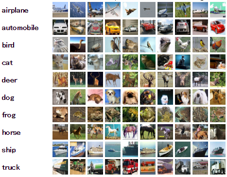
CIFAR-10 and CIFAR-100 datasets

基本的にやっていることはMNISTと変わりませんが、より実践的な内容となっており、精度を向上させる細かい工夫が各所にあるので、いろいろ紹介していきたいと思います。

チュートリアルのファイル構成

各ファイルの役割は、以下のようになっています。

cifar.py … 今回のCNNを構成する関数が格納されたファイル
cifar10_train.py … cifar.pyを使って実際に学習を実行するファイル
cifar10_eval.py … cifar10_train.pyで出力されたCNNを使って精度を確認するファイル

We hope that this tutorial provides a launch point for building larger CNNs for vision tasks on TensorFlow.

とのことなので、各アプリで"cifar.py"のようなものを設計・実装することが推奨されていると思われます。

この後は、以下の流れに沿って進めます。

入力データ準備
モデル構築
モデル学習
評価

1.入力データ準備 (cifar.distorted_inputs())

このチュートリアルでは、cifar.distorted_inputs()で、入力データを読み込むことができます。大筋の流れはMNISTの場合と同じですが、より実践に則したチュートリアルとなっており、以下の操作を行い学習データを増やしています。

32x32を24x24にトリミング tf.image.random_crop()
ランダムで左右逆転 tf.image.random_flip_left_right()
ランダムで明るさ変更 tf.image.random_brightness()
ランダムでコントラスト変更 tf.image.random_contrast()
画像の白色化（平均0と分散1に補正） tf.image.per_image_whitening()

なんと、この操作が全てTensorFlowのメソッドを呼び出すだけで、実行できるようになっています。

ディープラーニングは、画像認識の分野で発展したこともあり、この辺りの操作はすでにライブラリレベルでサポートされています。

さらっと記載しましたが、この分野についての手法提案からライブラリに載るまでの速度は、ハッキリ言って次元が異なります。素人がどうこうできるレベルを超えているので、ここは素直に恩恵にあずかりましょう。

2.モデル構築 (cifar.inference())

次に、cifar.inference()でモデルを構築します。

CNNについては、前回紹介しましたので、概要を軽く復習する程度にします。

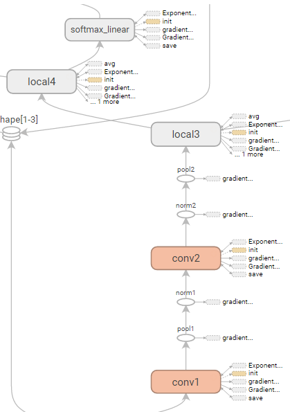
conv1, pool1, norm1, conv2, norm2, pool2, local3, local4, softmax_linearの10層で構成されています。

norm層は初出で、Local Response Normalization (LRN)層のことです。ReLU層の出力の正規化に用いられる操作で、doc stringによると以下の実装となってます

Local Response Normalization.
The 4-D `input` tensor is treated as a 3-D array of 1-D vectors (along the lastdimension), and each vector is normalized independently. Within a given vector, each component is divided by the weighted, squared sum of inputs within `depth_radius`. In detail,

sqr_sum[a, b, c, d] =
sum(input[a, b, c, d - depth_radius : d + depth_radius + 1] ** 2)
output = input / (bias + alpha * sqr_sum ** beta)

For details, see [Krizhevsky et al., ImageNet classification with deep
convolutional neural networks (NIPS 2012)]
(http://papers.nips.cc/paper/4824-imagenet-classification-with-deep-convolutional-neural-networks).

詳しくは、上記の[Krizhevsky+ 2012]の3.3節を参照ください。

あとは、日本語よりもコードを見たほうが早いので、引用します。

def inference(images):
  """Build the CIFAR-10 model.

  Args:
    images: Images returned from distorted_inputs() or inputs().

  Returns:
    Logits.
  """
  # We instantiate all variables using tf.get_variable() instead of
  # tf.Variable() in order to share variables across multiple GPU training runs.
  # If we only ran this model on a single GPU, we could simplify this function
  # by replacing all instances of tf.get_variable() with tf.Variable().
  #
  # conv1
  with tf.variable_scope('conv1') as scope:
    kernel = _variable_with_weight_decay('weights', shape=[5, 5, 3, 64],
                                         stddev=1e-4, wd=0.0)
    conv = tf.nn.conv2d(images, kernel, [1, 1, 1, 1], padding='SAME')
    biases = _variable_on_cpu('biases', [64], tf.constant_initializer(0.0))
    bias = tf.nn.bias_add(conv, biases)
    conv1 = tf.nn.relu(bias, name=scope.name)
    _activation_summary(conv1)

  # pool1
  pool1 = tf.nn.max_pool(conv1, ksize=[1, 3, 3, 1], strides=[1, 2, 2, 1],
                         padding='SAME', name='pool1')
  # norm1
  norm1 = tf.nn.lrn(pool1, 4, bias=1.0, alpha=0.001 / 9.0, beta=0.75,
                    name='norm1')

  # conv2
  with tf.variable_scope('conv2') as scope:
    kernel = _variable_with_weight_decay('weights', shape=[5, 5, 64, 64],
                                         stddev=1e-4, wd=0.0)
    conv = tf.nn.conv2d(norm1, kernel, [1, 1, 1, 1], padding='SAME')
    biases = _variable_on_cpu('biases', [64], tf.constant_initializer(0.1))
    bias = tf.nn.bias_add(conv, biases)
    conv2 = tf.nn.relu(bias, name=scope.name)
    _activation_summary(conv2)

  # norm2
  norm2 = tf.nn.lrn(conv2, 4, bias=1.0, alpha=0.001 / 9.0, beta=0.75,
                    name='norm2')
  # pool2
  pool2 = tf.nn.max_pool(norm2, ksize=[1, 3, 3, 1],
                         strides=[1, 2, 2, 1], padding='SAME', name='pool2')

  # local3
  with tf.variable_scope('local3') as scope:
    # Move everything into depth so we can perform a single matrix multiply.
    dim = 1
    for d in pool2.get_shape()[1:].as_list():
      dim *= d
    reshape = tf.reshape(pool2, [FLAGS.batch_size, dim])

    weights = _variable_with_weight_decay('weights', shape=[dim, 384],
                                          stddev=0.04, wd=0.004)
    biases = _variable_on_cpu('biases', [384], tf.constant_initializer(0.1))
    local3 = tf.nn.relu_layer(reshape, weights, biases, name=scope.name)
    _activation_summary(local3)

  # local4
  with tf.variable_scope('local4') as scope:
    weights = _variable_with_weight_decay('weights', shape=[384, 192],
                                          stddev=0.04, wd=0.004)
    biases = _variable_on_cpu('biases', [192], tf.constant_initializer(0.1))
    local4 = tf.nn.relu_layer(local3, weights, biases, name=scope.name)
    _activation_summary(local4)

  # softmax, i.e. softmax(WX + b)
  with tf.variable_scope('softmax_linear') as scope:
    weights = _variable_with_weight_decay('weights', [192, NUM_CLASSES],
                                          stddev=1/192.0, wd=0.0)
    biases = _variable_on_cpu('biases', [NUM_CLASSES],
                              tf.constant_initializer(0.0))
    softmax_linear = tf.nn.xw_plus_b(local4, weights, biases, name=scope.name)
    _activation_summary(softmax_linear)

  return softmax_linear

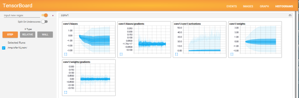
_activation_summary()で、各層の活性化後の値のヒストグラムと非ゼロ要素数を、サマリに追加しています。

これにより、TensorBoardでより多くの情報を確認することができます。

3.モデル学習

基本的に、以前ご紹介したMNISTの学習とやっていることは変わりませんが、少し工夫があります。

# 10反復毎に標準出力に情報を出力
if step % 10 == 0:
  num_examples_per_step = FLAGS.batch_size
  examples_per_sec = num_examples_per_step / duration
  sec_per_batch = float(duration)

  format_str = ('%s: step %d, loss = %.2f (%.1f examples/sec; %.3f '
                'sec/batch)')
  print (format_str % (datetime.now(), step, loss_value,
                       examples_per_sec, sec_per_batch))

# 100反復毎に、TensorBoardにサマリを出力
if step % 100 == 0:
  summary_str = sess.run(summary_op)
  summary_writer.add_summary(summary_str, step)

# 1000反復毎にモデルを保存
if step % 1000 == 0 or (step + 1) == FLAGS.max_steps:
  checkpoint_path = os.path.join(FLAGS.train_dir, 'model.ckpt')
  saver.save(sess, checkpoint_path, global_step=step)

特に、1000反復ごとにモデルを保存することにより、途中でCtrl+cで止めても学習途中のモデルが得られます。

Deep Neural Network（以下DNN）では、数日以上に渡ってモデルを学習することがあるので、定期的なシリアライズは時間を無駄にしないためにも重要です。

実際に実行したログはこちら

# python cifar10_train.py
>> Downloading cifar-10-binary.tar.gz 100.0%
Succesfully downloaded cifar-10-binary.tar.gz 170052171 bytes.
Filling queue with 20000 CIFAR images before starting to train. This will take a few minutes.
I tensorflow/core/common_runtime/local_device.cc:25] Local device intra op parallelism threads: 12
I tensorflow/core/common_runtime/gpu/gpu_init.cc:88] Found device 0 with properties:
name: Tesla K40c
major: 3 minor: 5 memoryClockRate (GHz) 0.745
pciBusID 0000:02:00.0
Total memory: 11.25GiB
Free memory: 11.15GiB
I tensorflow/core/common_runtime/gpu/gpu_init.cc:88] Found device 1 with properties:
name: Tesla K40c
major: 3 minor: 5 memoryClockRate (GHz) 0.745
pciBusID 0000:01:00.0
Total memory: 11.25GiB
Free memory: 11.15GiB
I tensorflow/core/common_runtime/gpu/gpu_init.cc:112] DMA: 0 1
I tensorflow/core/common_runtime/gpu/gpu_init.cc:122] 0:   Y Y
I tensorflow/core/common_runtime/gpu/gpu_init.cc:122] 1:   Y Y
I tensorflow/core/common_runtime/gpu/gpu_device.cc:643] Creating TensorFlow device (/gpu:0) -> (device: 0, name: Tesla K40c, pci bus id: 0000:02:00.0)
I tensorflow/core/common_runtime/gpu/gpu_device.cc:643] Creating TensorFlow device (/gpu:1) -> (device: 1, name: Tesla K40c, pci bus id: 0000:01:00.0)
I tensorflow/core/common_runtime/gpu/gpu_region_allocator.cc:47] Setting region size to 11377456333
I tensorflow/core/common_runtime/gpu/gpu_region_allocator.cc:47] Setting region size to 11377448551
I tensorflow/core/common_runtime/local_session.cc:45] Local session inter op parallelism threads: 12
2016-01-11 06:55:11.104789: step 0, loss = 4.68 (4.3 examples/sec; 29.519 sec/batch)
2016-01-11 06:55:13.824070: step 10, loss = 4.66 (554.8 examples/sec; 0.231 sec/batch)
2016-01-11 06:55:16.329406: step 20, loss = 4.64 (535.4 examples/sec; 0.239 sec/batch)
2016-01-11 06:55:18.885229: step 30, loss = 4.61 (516.3 examples/sec; 0.248 sec/batch)
2016-01-11 06:55:21.457211: step 40, loss = 4.60 (516.2 examples/sec; 0.248 sec/batch)
2016-01-11 06:55:23.996590: step 50, loss = 4.59 (520.7 examples/sec; 0.246 sec/batch)
2016-01-11 06:55:26.511654: step 60, loss = 4.57 (497.9 examples/sec; 0.257 sec/batch)
...

ドキュメントによると、4～5時間回すと大体86％の精度が出るとのこと。

sec/batchはブレインパッドの計算機の方が速い。さすがTesla K40c！！

ただし時間の都合上1時間で打ち切り、評価に移ります。

4.評価

今度はcifar10_eval.pyでモデルを評価していきます。こちらもMNISTの時と流れは同じですが、いくつか工夫があります。

まず、評価関数は、今回tf.nn.in_top_k()を使っています。正解が上位k個の予測の中に含まれる場合、各モデルの出力を正しいものとみなし、自動的にスコアします。

ただし今回はk=1なので、MNISTと最終的には同じ評価となっています。関数が用意されているのでtf.nn.in_top_k()を使用するのが無難でしょう。

ThreadingとQueues

さらに大きな工夫としては、評価もThreadingとQueuesを用いて、並列化しているところです。

TensorFlowではThreadingとQueuesを用いた並列計算を容易に行えるよう、tf.Coordinatorとtf.QueueRunnerというクラスが用意されています。

https://www.tensorflow.org/versions/master/how_tos/threading_and_queues/index.html

DNNではバッチを切って学習することや、メモリ空間がCPUとGPU双方にあり通信が必要なことから、キューイングしたいという要望は、多くあります。

特に、GPU側はメモリ空間に限りがあり、またGPUコアの番地の制限もあることから、TensorFlow側で処理をしてくれるのは、非常にありがたい話です。

今回は、実装の細かいところまで追えていないので、以下のチュートリアルの実装を書き写すことが第一手と思われます。

# Coordinatorを用意
coord = tf.train.Coordinator()
try:
  # キュー処理用のスレッド用意
  threads = []
  for qr in tf.get_collection(tf.GraphKeys.QUEUE_RUNNERS):
    threads.extend(qr.create_threads(sess, coord=coord, daemon=True,
                                     start=True))

  num_iter = int(math.ceil(FLAGS.num_examples / FLAGS.batch_size))
  true_count = 0  # Counts the number of correct predictions.
  total_sample_count = num_iter * FLAGS.batch_size
  # 評価処理を実行
  step = 0
  while step < num_iter and not coord.should_stop():
    predictions = sess.run([top_k_op])
    true_count += np.sum(predictions)
    step += 1

  # ここに同期処理がないので、バッチ内部を並列処理と思われる

  # Compute precision @ 1.
  precision = true_count / total_sample_count
  print('%s: precision @ 1 = %.3f' % (datetime.now(), precision))

  summary = tf.Summary()
  summary.ParseFromString(sess.run(summary_op))
  summary.value.add(tag='Precision @ 1', simple_value=precision)
  summary_writer.add_summary(summary, global_step)
except Exception as e:  # pylint: disable=broad-except
  coord.request_stop(e)

# スレッドの同期
coord.request_stop()
coord.join(threads, stop_grace_period_secs=10)